How to use the VLOOKUP function in Excel

VLOOKUP is one of the most useful functions in Excel. In fact, the world can be separated into two groups of people - those who know how wonderful VLOOKUP is, and those who haven't discovered it yet. This VLOOKUP tutorial will help you join the ranks of the enlightened.

VLOOKUP allows you to look up a value in a column of data, and then read across to another table and fetch that value. VLOOKUP is an incredibly versatile function which can be put to many different uses. Once you understand how to use it, you'll find all sorts of Excel problems you can solve with it. 

Here are some things that VLOOKUP is good for:

• Looking up the price of a product for a given product ID.
• Looking up the price of a product for a given sales quantity (i.e. you have a price sheet where the price per unit drops as more units are ordered)
• Finding the full name of an airport if you know the airport's three letter abbreviation
• Checking the date an employee started work, given the employee's staff ID number

The VLOOKUP function is particularly useful if you've been using multiple nested IF statements in situations like those described above, and you want an easier or more powerful way to get the same result. Be careful though - nested IF statements are still useful in places where the VLOOKUP statement can't help, so don't assume that VLOOKUP will solve everything for you.

VLOOKUP() Function Syntax

The VLOOKUP() function has the following syntax:

=VLOOKUP(lookup_value, lookup_table_range, column, exact)

VLOOKUP() works by taking the value you are looking up (lookup_value) and looking for it in the first column of the table you are searching in (lookup_table_range).

Once the function finds the matching value in the lookup_table_range, it then reads across that row the table to the column you chose and returns the value it finds there.

In some cases you want the VLOOKUP function to find the nearest match, and sometimes you'll want the exact match. In this function, exact is an optional value (that's why it's not shown in bold above). if you set the exact parameter to 1 the formula will look for the nearest value. If you set it to 0 (or leave it out), it will look for an exact match and return a #N/A error if it can't find an exact match.

Examples of the VLOOKUP() function in action - VLOOKUP with an exact match

Here is an example of how the VLOOKUP() function is used to find a value based on an exact match.

• Suppose you have a table that looks like the following:
  
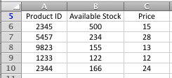
• You've been asked to come up with a way to check the price of a product when a product ID is typed into a given cell
• The formula you type in looks like this:
  
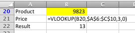
• In the table above, the VLOOKUP function looks for the value found in B20 (9823) in the first column of the range of cells from A6:C10 (i.e. the table in the previous step).
• Having found it in the first column (column A) it then reads across to the third column (column C) and retrieves the value. In this case, the value retrieved is 13.
• Some points to note about this scenario:
  
  • In case you're wondering, the $ signs in the function ($A$6:$C$10) mean that if you copy the formula in B21 to another location, it will continue to look in the product table. This is an example of absolute references in action; find out more about absolute references here. Note that if your VLOOKUP function generates a #N/A error, it could be because you didn't use absolute references, and then copied and pasted the VLOOKUP formula from one cell to another
  • No doubt you're sharp enough to have spotted the 0 as the exact, or fourth, parameter in the function in B21. This means that the VLOOKUP function is looking for an exact match. If it hadn't found the value from B20 (9823) in the first column of the table, the formula in B21 would have returned a #N/A error, meaning Excel couldn't return a value from the function. Remember, of course, that the exact parameter is optional, and defaults to 0 if you don't include it, so in this case we could have left this value out altogether and got the same result.
• If you want to become a VLOOKUP() ninja, here's something important you need to know about the exact parameter in the VLOOKUP function:
  
  • I'm sure you noticed this already, but did you see that the items in the Product ID table are not sorted in any order.
  • When using the VLOOKUP function, you need to check if the column you're performing the VLOOKUP on is sorted in ascending order (i.e. smallest values first, which means 1,2,3,4 or A,B,C,D). Sorting them in descending order (largest values first) isn't the same.
  • If the first column in your lookup table isn't sorted, you MUST use the exact version of the VLOOKUP function, as we did in this example. This forces the VLOOKUP() function to find an exact match. If an exact match cannot be found, the function will return a #N/A error.
  • If we had put 1 instead of 0 in our formula in the example above, the VLOOKUP function would have looked down the list in column A until either it found the value it was looking for, or it found a value that was larger than the value it was looking for, and then taken the previous value in column A as the nearest match. More on "nearest matches" with the VLOOKUP function in the next example.

Examples of the VLOOKUP() function in action - VLOOKUP with the nearest match

Here is an example of how the VLOOKUP() function is used to find a value based on an exact match.

• Suppose you have a table that looks like the following:
  
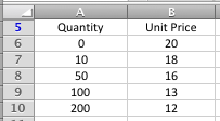
• This table represents a scenario where an order between 1 and 9 units will cost 20 per unit. An order between 10 and 49 units will cost 18 per unit, and so on.
  • It's important that you understand this before you go onto the next step, otherwise you'll get confused and the result the VLOOKUP function returns.
  • Note that in this scenario, any order over 200 units will cost 12 per unit.
  • We have also assumed that the minimum order quantity is greater than 0. However, the VLOOKUP function has no problem with using negative numbers if that's what your particular situation requires.
• In this example, you've been asked to come up with a way to check the price of a product for a given sales quantity. The method you choose should work for any sales quantity that is entered.
• You set up a VLOOKUP formula as follows:
  
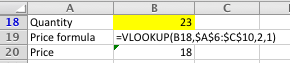
• The formula works by looking up the value in B18 (23) in the first column of the table (column A) in the previous step.
• Because the VLOOKUP() function is using the nearest match, it goes down column A looking for a match with the value in B18. In this example, it doesn't find one, and eventually it reaches the value in A8 (50) which the first value larger than the value it is looking for (23). At this point the VLOOKUP function stops looking and moves to the next step.
  • This is why, for VLOOKUP with a nearest match, you MUST sort the lookup table so the first column is in ascending order. If you don't, VLOOKUP may stop looking too soon, and ignore the possibility that a better (or exact) match existed further down the table.
• The VLOOKUP function then drops back to the previous row (10) and reads across the table to the second column and retrieves the value it finds (18).
• It's worth noting that it is very common when using the VLOOKUP table to get the design of the lookup table wrong. If your VLOOKUP function isn't working properly, check the design of the table first to make sure that it is correct.

As I said earlier, the VLOOKUP() function in Excel is very powerful. These are two examples of how to use it, but there are many more ways it can be applied. If you have a scenario where you think the VLOOKUP() function might apply but you can't figure it out, or you have another situation where you've successfully used the VLOOKUP() function in Excel, why not tell us about it the comments below?